User Guide

documentation

Introduction

1. Introduction

VesselAI is a unified digital twin and AI workspace designed specifically for maritime analytics.

It enables users to:

Analyze vessel performance and emissions
Process and explore AIS and telemetry datasets
Build optimization and predictive models
Automate workflows and create production pipelines

All directly from a web browser, without local setup.

2. Why Use VesselAI?

Modern maritime operations generate vast amounts of data:

AIS trajectories
Engine telemetry
Fuel consumption logs
Environmental and weather data

However, transforming this data into actionable insights requires more than just Python scripts. It requires:

A notebook environment
Data storage infrastructure
Pipeline orchestration
Model tracking
Version control and reproducibility

Setting up and maintaining this stack locally is complex and time-consuming.

VesselAI provides this entire infrastructure pre-configured and integrated.

You can focus on analysis and model development - not system administration.

3. What the Platform Provides

The VesselAI platform integrates the full analytics lifecycle into a single environment.

Tool	What it does	Why you need it
JupyterLab	Interactive notebook environment with pre-installed maritime libraries	Write Python notebooks, explore data, prototype models - no local setup required
Dagster	Pipeline orchestration engine	Schedule, monitor, and automate your notebook workflows with full observability
MLflow	Experiment tracking and model registry	Log metrics, compare runs, version models, and promote to production
MinIO	S3-compatible object storage	Store datasets, model artifacts, and output files in a centralized, shareable location
AI Model Library	Pre-trained maritime ML models	Ready-to-use models for CO₂ estimation, vessel position prediction, and more
Dashboard	Web UI for the entire platform	Monitor jobs, run inference, create pipelines - all from a single interface

These components work together — you do not need to configure them individually.

4. Key Advantages

No Local Setup

All dependencies, libraries, and configurations are already installed.

Centralized Data Storage

All datasets and results are stored in VesselAI Object Storage (MinIO).

Reproducible Workflows

Notebook runs and pipelines are tracked and versioned.

Collaboration

Users operate in a shared platform environment.

Security

Access is managed via Keycloak SSO and centralized authentication.

Maritime-Focused

The platform is tailored for vessel performance, emissions, routing, and optimization use cases.

Getting Started - Accessing the Platform

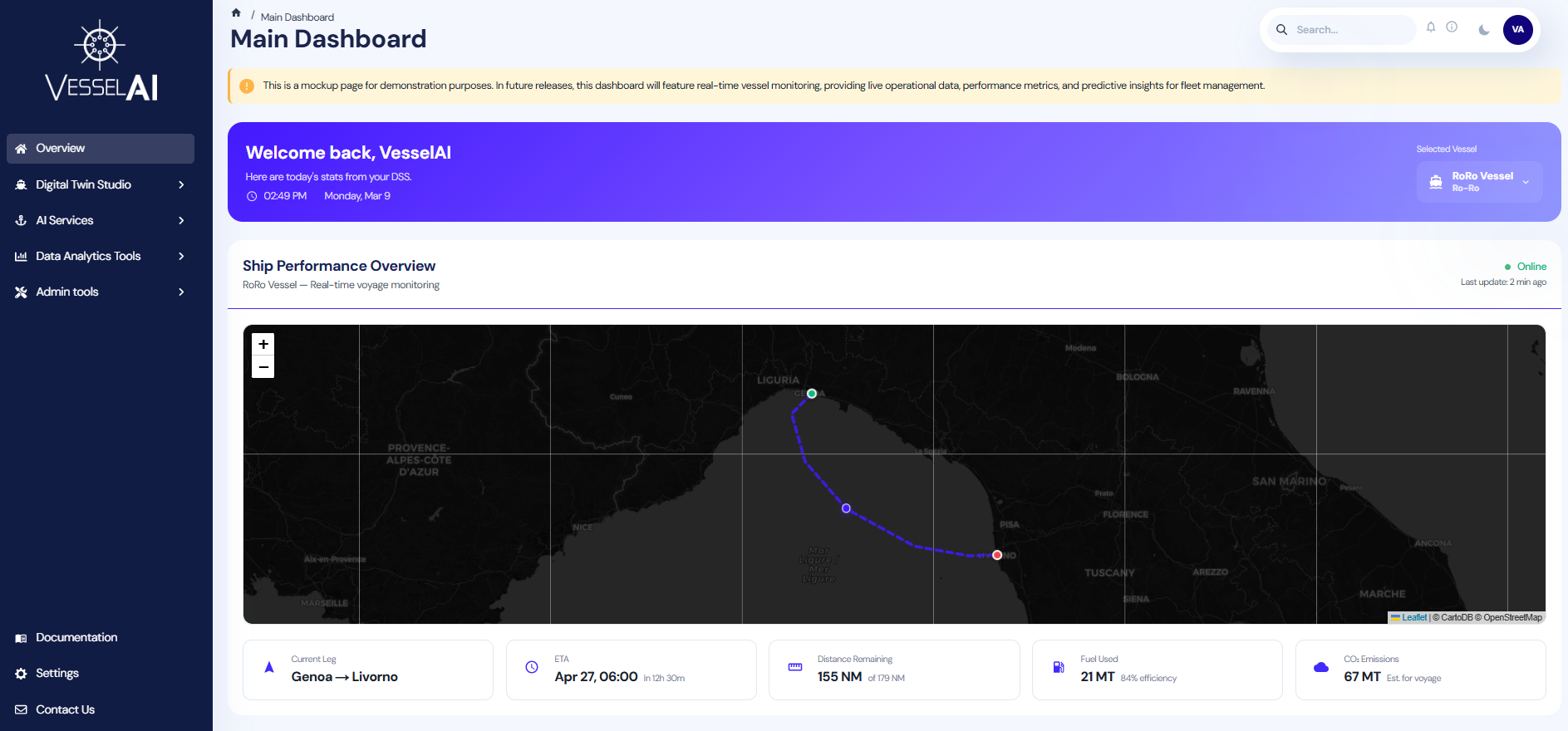
Navigate to the VesselAI platform URL provided by your administrator. Log in with your Keycloak credentials. You will land on the Dashboard, which provides access to all platform tools via the sidebar.

Platform Workflow Examples

The following sections present practical, end-to-end workflows that demonstrate how the core components of the VesselAI platform work together.

Each workflow is designed as a guided example, helping you move from data to results using real platform features.

Example 1: Mooring Analysis Pipeline - Chaining Jobs

Platform tools used in this example: Notebook Environment, Object Storage, AI Workflows (observational mode)

Objective

This workflow demonstrates how to:

Execute two analytical notebooks as independent jobs
Convert them into Dagster observational jobs
Chain them into a structured pipeline
Create a repeatable maritime analytics workflow

The goal of this pipeline is to:

Preprocess mooring-related vessel and environmental data
Perform optimization analysis on mooring configurations

Conceptual Overview

The pipeline consists of two notebooks:

1. Mooring Preprocessing Notebook

mooring_preprocessing.ipynb

Purpose:

Load raw mooring-related datasets
Clean and validate sensor inputs
Perform feature engineering
Store processed data in Object Storage

Output:

Structured dataset ready for optimization

2. Mooring Optimization Notebook

mooring_optimization.ipynb

Purpose:

Load preprocessed dataset
Apply optimization logic
Evaluate mooring configurations
Output optimal solution and diagnostics

Output:

Optimized mooring parameters
Performance metrics
Result artifacts saved to Object Storage

Each notebook performs a complete analytical stage.

In this example, we will execute each notebook as a single asset (Observational Mode).

Step 1 - Create Observational Jobs

Navigate to:

AI Services → Notebook Environment

A. Create Mooring Preprocessing Job

Locate:
```
mooring_preprocessing.ipynb
```
Before linking the notebook to Dagster, users can open it to examine the preprocessing workflow, including data loading, cleaning, and feature engineering steps.
Click the Link to Dagster Job icon.
Select:
```
Observational Mode
```
and click:
```
Link
```

In Observational Mode:

The entire notebook is executed as one asset.
The notebook runs sequentially.
Logs and execution status are tracked in Dagster.

The job will now appear in:

AI Services → Workflows

B. Create Mooring Optimization Job

Repeat the same process:

Locate:
```
mooring_optimization.ipynb
```
Click Link to Dagster Job
Select:
```
Observational Mode
```
and click:
```
Link
```

Now you have two independent jobs:

Mooring Preprocessing
Mooring Optimization

Each job can be executed separately.

Step 2 - Create a Chain Job

Now we create a pipeline that executes both jobs in sequence.

Navigate to:

AI Services → AI Workflows

Create New Chain Job

Click Create chain
Select:
- Step 1 → Mooring Preprocessing Job
- Step 2 → Mooring Optimization Job

This defines execution order:

Preprocessing → Optimization

Click:
```
Create Chain
```
and name you chain job:
```
mooring_chain_pipeline
```
Click:
```
Create
```
Your new chain job appears in the job list with a "Chain" badge.

Step 3 - Execute the Chain Job

After creating the chain job:

Click:

Run

The platform will automatically redirect you to the Dagster UI

Step 4 - Launch the Run in Dagster

After clicking Run, you are redirected to the Dagster UI.

In Dagster:

Click Launch Run (bottom right corner).
The pipeline execution will begin.

You will see the job executing sequentially:

mooring_preprocessing_job → mooring_optimization_job

During execution, you can:

Monitor the status of each step
View real-time logs
See execution duration
Identify any errors (if they occur)

The second step (optimization) will start automatically after the preprocessing step completes successfully.

Once both steps finish, the run status will appear as:

Success

Step 5 - View Results in AI Workflows

After the chain job has successfully completed in Dagster:

Navigate back to:
```
AI Services → AI Workflows
```
Locate your chain job:
```
Mooring Chain Pipeline Chain Job
```
Click View Results

What You Will See

The Results view provides a structured summary of the latest execution:

Pipeline Overview

Execution status (Success / Failed)
Execution timestamp
Total duration
Number of steps
Visual pipeline diagram showing:
- Step 1 → Mooring Preprocessing
- Step 2 → Mooring Optimization

This confirms that both stages executed sequentially.

Step Details

Each step can be expanded to show:

Notebook used
Execution duration
Generated output tables
Handoff information between steps

For example:

Step 1 – Mooring Preprocessing

Output dataset saved to Object Storage
Displays the bucket and storage key of the processed file

Step 2 – Mooring Optimization

Displays generated result tables (e.g., polygons_csv)
Shows final output artifacts

Output Tables

The final section displays the pipeline output:

chain_output (CSV – Primary)

This represents the final result of the entire chain job and originates from the optimization stage.

What Happens During Execution

When the chain job runs:

1️. The preprocessing notebook executes:

Raw data is cleaned
Features are engineered
Processed dataset is saved to Object Storage

The optimization notebook executes:

Loads processed dataset
Performs optimization logic
Saves final results

Dagster ensures:

Sequential execution
Failure handling
Log tracking
Execution monitoring

Example 2 - Train and Use a CO₂ Emissions Model

Platform tools used in this example: AI Workflows, MLFlow (internal only), Notebook Environment, Object Storage

Objective

In this workflow, you will:

Run a predefined Dagster job to train a CO₂ emissions model
Track and register the model in MLflow
Retrieve the trained model inside a Notebook
Perform predictions on voyage data
Visually compare predicted vs actual emissions

This demonstrates a complete AI lifecycle within VesselAI:

Data → Training → Model Registry → Inference → Validation

Part 1 - Train the CO₂ Emissions Model

Step 1 - Open the Training Job

Navigate to:

AI Services → AI Workflows

Locate the card:

Co2 Emissions Training Job

Click:

Run Now

This opens the Dagster job page.

You will see the three pipeline assets:

input_data → trained_model → evaluated_pipeline

These represent:

Loading training data -> Training the model -> Evaluating and logging results

Step 2 - Launch the Configuration

Click:

Materialize All

This opens the Dagster Launchpad configuration editor.

Step 3 - Configure the Run

The Launchpad pre-fills the following configuration:

ops:
  co2__train__evaluated_pipeline:
    config:
      co2_model_name: co2_rfr

  co2__train__input_data:
    config:
      bucket: co2-data
      filename: bulk-cleaned-voyage-data.csv

  co2__train__trained_model:
    config:
      model:
        mlp:
          activation: relu
          alpha: 0.001
          hidden_layer_sizes:
            - 100
            - 50
          max_iter: 1000
          solver: adam

        rfr:
          n_estimators: 100

⚠ Important: You must keep only one model block: Either mlp Or rfr. Delete or comment out the model you do not want to use. If both remain, Dagster will show: You can only specify a single field at path (...config.model). Name your model respectively, for example for rfr keep: co2_model_name: co2_rfr

Step 4 - Optional Customization

You may adjust:

bucket → MinIO bucket containing training data
filename → Voyage dataset CSV
Model hyperparameters

Step 5 - Launch Training

Click:

Materialize

The pipeline will:

Load voyage data from MinIO
Train the selected model (MLP or Random Forest)
Evaluate model performance
Log metrics and artifacts to MLflow
Register the model

Step 6 - View Results

Once the run completes:

Return to:

AI Services → AI Workflows

Click:

View Results

You will see:

Metrics (e.g. MAE, RMSE)
Model version
Model name
Parameters (e.g. Dataset, features)

Note the following: Model Name, Model Version. You will use these in the next section.

Part 2 - Load and Use the Trained Model

Now we switch from orchestration to analysis.

Step 7 - Open Notebook Environment

Navigate to:

AI Services → Notebook Environment

Create a new notebook:

co2_inference_example.ipynb

Select the Python kernel.

Step 8 - Import Required Utilities

import pandas as pd
import matplotlib.pyplot as plt

from utils.minio_helper import minio, mlflowx

Step 9 - Load the Registered Model

Use the model name and version observed in View Results:

model = mlflowx.load_model(
    model_name="co2_rfr_model",   # replace with your model name
    version=1                    # replace with your model version
)

print(model)

The model is now loaded directly from the MLflow Model Registry.

Step 10 - Load Voyage Data

data = minio.read_csv("co2-data/bulk-cleaned-voyage-data.csv") #or upload the path to your data

Select features used during training:

features = [
  "imo",
  "v_draft",
  "v_departure_lat",
  "v_departure_lon",
  "v_arrival_lat",
  "v_arrival_lon",
  "seapassage_distance[m]",
  "seapassage_duration[s]",
  "seapassage_avg_speed[m/s]",
  "time_bf0",
  "time_bf1",
  "time_bf2",
  "time_bf3",
  "time_bf4",
  "time_bf5",
  "time_bf6",
  "time_bf7",
  "time_bf8",
  "time_bf9",
  "time_bf10",
  "time_bf11",
  "time_bf12"
]

X = data[features]

Step 11 - Run Predictions

predictions = model.predict(X)

Select the last 50 samples for visualization:

n = 50
y_pred = predictions[-n:]
y_true = data["co2[kg]"].to_numpy()[-n:]

x = range(n)
Step 12 - Visualize Performance
plt.figure()
plt.plot(x, y_pred, label="Predicted CO2 [kg]")
plt.plot(x, y_true, label="Actual CO2 [kg]")
plt.legend()
plt.title("Predicted vs Actual CO₂ Emissions")
plt.show()

You now have a visual validation of model performance.

Example 3 - Full Mooring Pipeline

Platform tools used in this example: Notebook Environment, Object Storage, AI Workflows (pipeline mode)

Objective

In this workflow, you will:

Inspect a structured pipeline notebook
Link it to Dagster in Pipeline Mode
Visualize step-level assets
Execute the pipeline
Review outputs and artifacts

Unlike the previous example (Observational Mode), here:

Each # %% step: block becomes an independent Dagster asset.

Step 1 - Navigate to the Notebook Environment

Go to:

AI Services → Notebook Environment

Locate:

mooring_pipeline.ipynb

Step 2 - Inspect the Notebook Structure

Open the notebook and review the code.

You will notice that the notebook contains special directives such as:

# %% step: setup

Each # %% step: defines a pipeline stage.

For example:

# %% step: setup

This step:

Loads configuration parameters
Defines MinIO input/output paths
Sets optimization controls
Configures environment variables

Other steps in the notebook include:

Data loading from Object Storage
Mooring data preprocessing
Optimization logic
Saving results back to Object Storage
Generating output artifacts

These steps:

Use minio.read_csv() to load AIS data
Use minio.write_csv() to store results
Pass intermediate data between steps
Generate structured outputs

Step 3 - Link Notebook as a Pipeline Job

Return to the Notebook Environment list.

Click the Link to Dagster Job icon.

In the execution mode dialog:

Select:

Pipeline Mode

Then click:

Link

This tells the platform:

Parse # %% step: blocks
Register each step as a Dagster asset
Create a structured pipeline job

Step 4 - Locate the Pipeline in AI Workflows

Navigate to:

AI Services → AI Workflows

Find the newly created job:

Mooring Pipeline Job

Click the following badge, located under the job's name to open the job details :

mooring_pipeline_job

You are now redirected to Dagster UI, where you can see the assets defined in Jupyterlab notebook.

Step 5 - Launch the Pipeline in Dagster

In the Dagster interface navigate to:

Launchpad

Click (bottom right) :

Launch Run

What You Will See in Dagster

Dagster will display:

A visual asset graph
Each # %% step: as a separate node
Execution progressing sequentially
Logs for each step

Each step:

Executes independently
Has its own logs
Produces its own outputs
Passes data to downstream steps

This provides:

Fine-grained observability
Step-level failure isolation
Re-execution capability per asset

Step 6 - Return to AI Workflows

After successful execution:

Navigate back to:

AI Services → AI Workflows

Locate:

Mooring Pipeline Job

Click:

View Results

What You Can Review in Results

Pipeline Summary
- Status (Success)
- Execution timestamp
- Step breakdown
- Total duration

Step-Level Outputs

Each step displays:
- Output tables
- Stored CSV files
- Object Storage locations (S3 paths)
- Execution parameters
Example outputs:
```
preprocessed_csv  → s3://ais-data/preprocessed/...
polygons_csv      → s3://ais-data/optimized/...
```

Parameters Section

You can also review:
- Execution configuration
- Environment overrides
- Input bucket / filename
- Runtime settings (e.g., GA generations)

Platform tools used in this example: Notebook Environment, Object Storage, AI Workflows (observational mode)

Objective

This workflow demonstrates how to:

Link an analytical notebook to Dagster in Observational Mode
Execute it as a single job
View results in a structured results card
Share model performance outputs in a centralized interface

This approach is ideal when:

You want to expose results without exposing code
You want a clean summary view for collaborators
You want reproducible execution tracking

Use Case - Fuel Consumption Predictor

The notebook used in this example:

fuel-consumption-predictor.ipynb

This notebook:

Trains a fuel consumption prediction model
Evaluates performance using MAE, MSE, and R²
Generates diagnostic plots
Produces structured performance metrics

This enables:

Validation of fuel efficiency models
Comparison between predicted and actual consumption
Identification of data distribution patterns
Performance benchmarking

Results are exposed through a standardized job result card.

Step 1 - Navigate to Notebook Environment

Go to:

AI Services → Notebook Environment

Locate:

fuel-consumption-predictor.ipynb

You may open the notebook to review:

Data preprocessing logic
Model training
Evaluation metrics
Visualization generation

Step 2 - Link Notebook to Dagster

Click the Link to Dagster Job icon.

Select:

Observational Mode

Click:

Link

What Observational Mode Does

Executes the entire notebook as one asset
Preserves notebook execution order
Tracks logs and execution status
Produces a structured result card

No pipeline structure is required.

Step 3 - Run the Job

Navigate to:

AI Services → AI Workflows

Locate the newly created job card:

Fuel Consumption Predictor Job

Click:

Run

You will be redirected to the Dagster UI.

Click:

Launch Run

The notebook executes fully.

Step 4 - View Results

After successful execution:

Return to:

AI Services → AI Workflows

Click:

View Results

What You Will See in the Results Card

The results card presents:

Execution Summary
- Status (Success)
- Notebook name
- Execution timestamp
Metrics

Displayed clearly in structured format:
- MAE
- MSE
- R²
- Additional evaluation metrics (e.g., R² without CO₂)

These metrics provide an immediate understanding of model accuracy.

Plots

The card displays generated visual diagnostics, including:

Distribution histograms
Correlation heatmap
Boxplots of numerical variables
Fuel and CO₂ distribution comparisons

This provides:

Quick model validation
Outlier detection visibility
Variable relationship insight
Parameters

Expandable section showing:

Model configuration
Execution parameters
Hyperparameters used

Introduction​

1. Introduction​

2. Why Use VesselAI?​

3. What the Platform Provides​

4. Key Advantages​

No Local Setup​

Centralized Data Storage​

Reproducible Workflows​

Collaboration​

Security​

Maritime-Focused​

Getting Started - Accessing the Platform​

Platform Workflow Examples​

Example 1: Mooring Analysis Pipeline - Chaining Jobs​

Objective​

Conceptual Overview​

Step 1 - Create Observational Jobs​

A. Create Mooring Preprocessing Job​

B. Create Mooring Optimization Job​

Step 2 - Create a Chain Job​

Create New Chain Job​

Step 3 - Execute the Chain Job​

Step 4 - Launch the Run in Dagster​

Step 5 - View Results in AI Workflows​

What You Will See​

What Happens During Execution​

Example 2 - Train and Use a CO₂ Emissions Model​

Objective​

Part 1 - Train the CO₂ Emissions Model​

Part 2 - Load and Use the Trained Model​

Example 3 - Full Mooring Pipeline​

Objective​

Step 1 - Navigate to the Notebook Environment​

Step 2 - Inspect the Notebook Structure​

Step 3 - Link Notebook as a Pipeline Job​

Step 4 - Locate the Pipeline in AI Workflows​

Step 5 - Launch the Pipeline in Dagster​

Step 6 - Return to AI Workflows​

Example 4 - Share Model Results via Observational Notebook Job​

Objective​

Step 1 - Navigate to Notebook Environment​

Step 2 - Link Notebook to Dagster​

Step 3 - Run the Job​

Step 4 - View Results​

Introduction

1. Introduction

2. Why Use VesselAI?

3. What the Platform Provides

4. Key Advantages

No Local Setup

Centralized Data Storage

Reproducible Workflows

Collaboration

Security

Maritime-Focused

Getting Started - Accessing the Platform

Platform Workflow Examples

Example 1: Mooring Analysis Pipeline - Chaining Jobs

Objective

Conceptual Overview

Step 1 - Create Observational Jobs

A. Create Mooring Preprocessing Job

B. Create Mooring Optimization Job

Step 2 - Create a Chain Job

Create New Chain Job

Step 3 - Execute the Chain Job

Step 4 - Launch the Run in Dagster

Step 5 - View Results in AI Workflows

What You Will See

What Happens During Execution

Example 2 - Train and Use a CO₂ Emissions Model

Objective

Part 1 - Train the CO₂ Emissions Model

Part 2 - Load and Use the Trained Model

Example 3 - Full Mooring Pipeline

Objective

Step 1 - Navigate to the Notebook Environment

Step 2 - Inspect the Notebook Structure

Step 3 - Link Notebook as a Pipeline Job

Step 4 - Locate the Pipeline in AI Workflows

Step 5 - Launch the Pipeline in Dagster

Step 6 - Return to AI Workflows

Example 4 - Share Model Results via Observational Notebook Job

Objective

Step 1 - Navigate to Notebook Environment

Step 2 - Link Notebook to Dagster

Step 3 - Run the Job

Step 4 - View Results